Interpolation Tool
Introduction
For an attribute collected at several point features, such as nitrate measured
at marine monitoring stations, proportional symbols will depict the nitrate
level at specific stations. This is good for visualizing general spatial patterns
in the data, but gaps in the spatial coverage of this data remain. The interpolation
tool helps to fill these gaps. The interpolation tool is designed to
be used with point attribute data. To activate the tool, make the point data
source active in the Layer Manager. Then press the interpolation tool
icon ![]() to display the interface, where
various parameters can be changed.
to display the interface, where
various parameters can be changed.
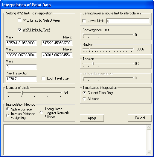
Spatial Parameters
This section of the interface allows the user to change the spatial bounds for interpolation in two or three dimensions. Within those limits the resolution of the interpolated raster output can be defined.
There must be seven or more data values within the defined area for interpolation to take place.
This uses the Select Box to define the x (East-West) and y (North-South) extent for interpolation. The user must ensure that the Select Box is positioned correctly before invoking the interpolation tool.
Spatial Extent Defined by Text
As default, the limits of the point data in the x and y dimensions are displayed in the text boxes.
The interpolated raster output must be a square image and the size must be a power of 2 (i.e. 16, 32, 64, 128, 256, 512, 1024, 2048 or 4096). The user can change the default of 64 pixels by using the slider. If the select area or the user text-specified interpolation area is not square then the interpolation area will be extended to the north or east to produce a square in map co-ordinates.
This allows the setting of limits to the interpolated output. For instance, this tool can interpolate negative values, unless a lower limit of zero is set. Whilst negative values may be possible with attributes such as temperature, a negative nitrate value is clearly wrong.
The user can optionally insert a value for the lower attribute limit. The default is zero.
There are three interpolation methods available. The default is the minimum curvature method devised by W.H.F. Smith and P.Wessel (see copyright statement below). For more details about the method, and more specifically the three changeable parameters in this tool; convergence, radius and tension, consult the following reference:
W.H.F. Smith & P.Wessel (1990), "Gridding with continuous curvature splines in tension" in Geophysics, Vol.55, No.3, p.293-305.
The two remaining methods are the Inverse Distance Weighting method and the Triangulated Irregular Network. Each method has its own advantages for certain datasets.
The minimum curvature method uses a number of parameters:
The interpolated output is reached through multiple iterations, with each iteration converging towards a solution. The interpolated value at each pixel changes with each successive iteration. When the change between iterations falls below the convergence limit, a solution has been reached. The default value is 0.
There are many rounds of iteration. Initially, a coarse lattice (superimposed on the original grid and at least 4 x 4 in dimension) has to be seeded with values. With a grid of larger dimension, the values in the coarse lattice are seeded to zero. However with a smaller grid whose dimension approaches that of the coarse lattice, values can be calculated by weighted average. In this case, a radius is defined around each point in the coarse lattice, and real data points falling within this radius are weighted according to their inverse distance from the coarse lattice point, then averaged. The default radius is zero.
Convergence towards a solution for the coarse lattice follows, with the output being fed into a finer lattice, which itself is iterated to convergence. This process continues until the dimensions of the coarse lattice assumes that of the original grid.
Use of the minimum curvature method can result in large oscillations and dubious inflection points on the output surface. Imagine the surface as an elastic plate stretched and deformed so that it fitted all the input data points. The use of tension on this surface minimizes the oscillations and inflection points, making for a more realistic fit. Tension ranges from 0 (no tension) to just less than 1 (maximum tension). The default value is 0.2.
Time-based Interpolation
If the current layer, chosen for interpolation, contains more than one time slice then the user has the option to perform a multi-temporal interpolation. This will perform an interpolation for each time slice in the current layer and will create a new layer containing all of these interpolated time slices.
To select a multi-temporal interpolation click on the All times option.
Note: This facility does not perform a temporal interpolation between time slices in the original layer.
Once all parameters have been changed to your satisfaction, click on Apply to start the interpolation. Alternatively you can click Cancel to exit the interpolation tool at any time.
Example of Interpolation Output
Finally, a word of warning. The interpolation tool is designed for exploration only, and must be used sensibly if it is expected to produce useful output. These are cases in point:
Interpolated attribute error is proportional to the distance from real data points. Therefore, a dense, evenly spaced point input data set is optimal. Avoid large empty areas either within or outside of the main body of data.
It is recommended that the level of tension for data should be approximately 0.25. Topography may require a higher level of tension.
Copyright Statement for the Interpolation Calculation Software
Copyright © 1991-1995, P. Wessel & W. H. F. Smith
Permission to use, copy, modify, and distribute this software and its documentation for any purpose without fee is hereby granted, provided that the above copyright notice appear in all copies, that both that copyright notice and this permission notice appear in supporting documentation, and that the name of GMT not be used in advertising or publicity pertaining to distribution of the software without specific, written prior permission. The University of Hawaii (UH) and the National Oceanic and Atmospheric Administration (NOAA) make no representations about the suitability of this software for any purpose. It is provided "as is" without expressed or implied warranty. It is provided with no support and without obligation on the part of UH or NOAA, to assist in its use, correction, modification, or enhancement.
| Browser Based Help. Published by chm2web software. |